
Nine engineering constants define an orthotropic compliance in material axes; the response is transformed to the global frame.
01 Model and scope
A homogeneous orthotropic solid has three preferred perpendicular material axes and nine independent engineering constants. QF Solver constructs the symmetric compliance in those axes, requires it to be positive definite, solves for stiffness, then rotates strain into and stress out of the declared material frame.
Route assumptions and calculation checks
- Nine constants define one homogeneous small-strain 3D law; reciprocity determines ν21, ν31, and ν32.
- The 6×6 compliance must be symmetric positive definite; Q must be orthonormal and right-handed.
- Current owner-accepted scope covers bounded linear-static TET4/TET10 cases. Modal/dynamic/large-model wiring remains separately evidenced; this is not a 3D delamination model.
Useful foundations and prerequisites
02 Essential equations and symbols
Definitions and conventions
- Young moduli along material axes 1, 2, and 3.
- Poisson ratios in the QF Solver input convention; reciprocal terms follow elastic symmetry.
- Shear moduli in the corresponding material planes.
- Compliance and stiffness in engineering-Voigt order [11,22,33,12,23,13].
- 3×3 orthonormal, right-handed orientation matrix whose columns are material axes in global coordinates.
03 Step by step derivation
Follow the assumptions, equations and discrete operations in order. The full explanation stays visible.
This is a 3D small-strain solid law. It is distinct from the plane-stress orthotropic lamina used by the laminate cards: the latter has in-plane axes 1–2 and a separate thickness-shear model. Material orientation is a physical input, not a display setting.
1 · Define material axes and independent constants
The material coordinate frame follows the local microstructure: axis 1 might follow fibres, axis 2 the in-plane transverse direction, and axis 3 the solid thickness direction. A single set of nine moduli assumes the material is uniform within the element and that the orthotropic axes remain fixed there.
The code accepts a global frame, a 3×3 orientation, or an e₁ direction plus an orthogonalizing hint. A cylindrical-tangent field is evaluated at an element centroid; it does not resolve arbitrary fibre steering within an element.
2 · Enforce reciprocal Poisson coupling
The six axial normal compliances and three shear compliances form a symmetric 6×6 matrix. Symmetry imposes reciprocal Poisson ratios; they are not extra independent inputs. In the declared convention, νᵢⱼ is entered for the transverse strain in j under loading along i.
The off-diagonal terms are negative under the usual positive Poisson-ratio convention. The code checks positive definiteness of Sₘ rather than relying on independent positivity of Eᵢ and Gᵢⱼ alone.
3 · Invert compliance and test elastic stability
The stiffness is obtained by solving SₘDₘ=I and symmetrizing round-off. Positive definiteness means positive strain energy for every non-zero admissible strain. It is a material admissibility test; it does not validate units, manufacturing data, element interpolation, or mesh quality.
A matrix that passes this check can still describe an unmeasured or poorly identified material. Material constants need test provenance and a consistent unit system.
4 · Rotate the tensor law without losing shear factors
Let Q contain the material basis vectors as columns in global coordinates. Global strain is transformed as QᵀεgQ, the constitutive law is applied in material axes, and the resulting stress is transformed back as QσmQᵀ. The implementation converts through symmetric tensors so the engineering-shear factors are applied explicitly.
Rotating a 6×6 matrix by a generic 3×3 formula is error-prone because stress and engineering strain Voigt vectors transform differently. The code applies and tests the tensor rotations instead.
5 · Where the current evidence applies
The cited specification accepts bounded linear-static TET4 and TET10 cases for internal engineering use, with recommendations. It also describes modal, Newmark, and large-model wiring, but those additional paths remain development until their own benchmark and review requirements close.
No 3D composite failure criterion is computed by this law. It is not a ply-stack delamination model, a nonlinear orthotropic law, or a continuously varying orientation field.
04 Algorithm and implementation
Source excerpt · v0.2.11
The implementation builds reciprocal compliance in material axes, solves for stiffness, and rotates strain/stress through tensor form so engineering shear factors are preserved.
Functions shown: material_elasticity_matrix stress_tangent strain_material_axes
@cached_property
    def material_elasticity_matrix(self) -> np.ndarray:
        matrix = np.linalg.solve(self.compliance_matrix, np.eye(6))
        return 0.5 * (matrix + matrix.T)

    def stress_tangent(self, strain):
        tangent = self.elasticity_matrix
        return tangent @ np.asarray(strain, dtype=float), tangent

    def strain_material_axes(self, global_strain):
        tensor = strain_voigt_to_tensor(global_strain)
return strain_tensor_to_voigt(self.orientation.T @ tensor @ self.orientation)05 Verification and limitations
OWNER-ACCEPTED BOUNDED SCOPE · material axes required
TET4/TET10 linear-static orthotropic cases are documented; dynamics and composite scopes remain route-specific.
Each reference supports its own model, observable and analysis route. Read the original contract and limitations before transferring a conclusion.
See this method in a calculation.
Each case keeps its mesh, measured quantities, source record and limitations attached to the result.
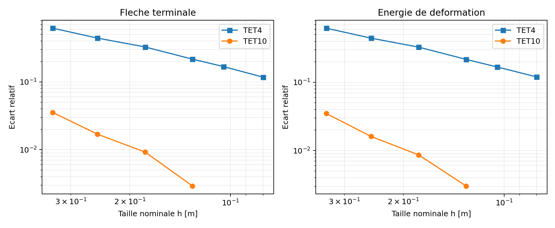 VNV-ORTHOTROPIC-SOLID-CONVERGENCE-003Orthotropic solid mesh convergenceTET10 deflection error: 0.292%Read model, result and limits →
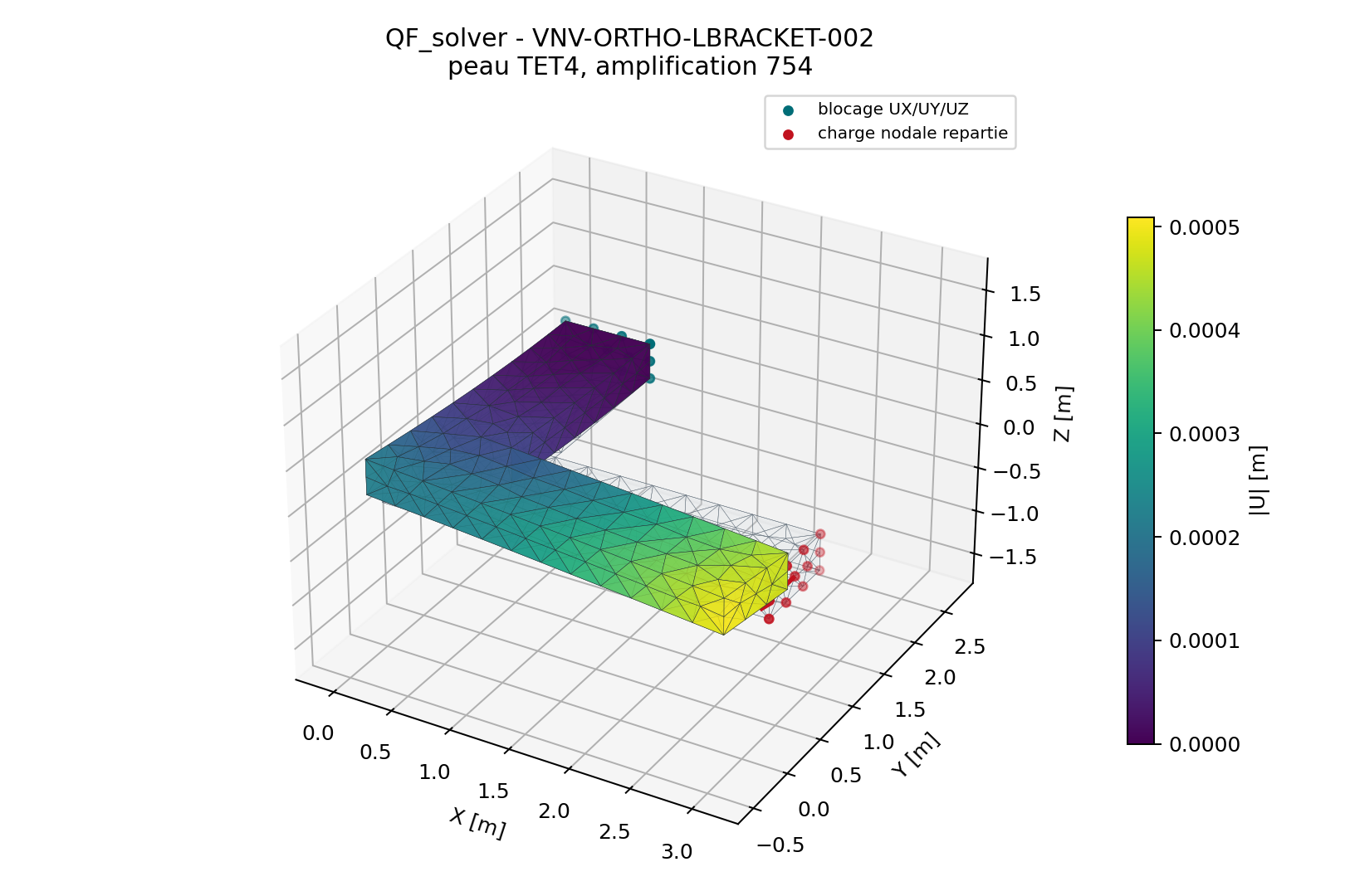 VNV-ORTHOTROPIC-SOLID-EXTERNAL-002Orthotropic bracket and perforated specimen correlationPerforated field difference: 0.000132% / 3.60 × 10⁻¹¹%Read model, result and limits →