Bilinear Q4 midsurface interpolation, six nodal DOFs, membrane, bending, transverse shear, and a weak drilling stabilizer.
01 Model and scope
Reissner–Mindlin kinematics retain transverse shear by allowing rotations independent of the midsurface slope. MITC4 samples covariant shear at tying points and interpolates it across the element; membrane, bending, shear and drilling terms remain distinct contributions.
Route assumptions and calculation checks
- MITC tying points interpolate covariant transverse shear to reduce shear locking.
- The drilling term is a weak penalty and requires sensitivity checks.
- Maturity remains specific to analysis, mass, damping, laminate, and benchmark route.
Useful foundations and prerequisites
02 Essential equations and symbols
Definitions and conventions
- Midsurface translations.
- rₓ,rᵧ
- Section rotations about the local axes.
- Membrane strain, curvature and transverse shear.
- A, Db, S
- Section matrices for membrane, bending and shear response.
03 Step by step derivation
Follow the assumptions, equations and discrete operations in order. The full explanation stays visible.
1 · Flat facet, local frame, and six DOFs per node
MITC4 is a four-node Reissner–Mindlin shell facet. Each corner carries local midsurface translations (u₀,v₀,w₀) and rotations (rₓ,rᵧ,r_z); the local basis is built from the facet diagonals and then nodal DOFs are transformed between local and global frames. Four nodes give 24 element DOFs.
Rotations remain independent of the slope of w. That permits transverse shear, unlike Kirchhoff–Love kinematics.
2 · Separate membrane, curvature, and shear energy
The in-plane strain changes linearly through thickness; integrating the isotropic plane-stress law gives extensional, bending, and shear resultants. With t the thickness, E and ν material constants, and κₛ a shear correction, membrane stiffness scales with t, bending stiffness with t³, and shear stiffness with t.
The sign of curvature and the top/bottom stress labels follow the oriented local normal; reversing the facet orientation changes those labels.
3 · MITC tying field and shear locking
Direct bilinear interpolation of transverse shear can over-constrain a thin shell as t/L becomes small. MITC4 samples covariant shear at four tying points: A and C for the ξ component, D and B for the η component. Linear interpolation across the opposite parent coordinate constructs the assumed shear field, which is then mapped to physical components by the surface Jacobian.
The tying operator is the central MITC step. It is not a general cure for every distortion or shell boundary-layer error; patches, thin-shell benchmarks, and mesh refinement remain necessary.
4 · Element stiffness, drilling stabilization, and integration
The local 24×24 stiffness is accumulated as separate membrane, bending, shear, and drilling terms at four 2×2 Gauss points. r_z is a drilling rotation rather than a physical thin-shell kinematic; a weak penalty stabilizes it and must not dominate the physical energy. Local stiffness is transformed back to global DOFs.
The implementation exposes stiffness components separately, making drilling-energy sensitivity inspectable. Four-point integration applies to this documented route.
5 · Mass, evidence, and limits
The consistent shell mass carries surface inertia ρt for translations and rotary inertia ρt³/12 for rₓ,rᵧ. Drilling rotation has zero physical inertia and is deliberately massless; a reducer handles those DOFs where needed. Verification separates membrane, bending and shear patches, thin-shell locking studies, Cook, Scordelis–Lo, pinched cylinder, modal and dynamic cases. The card's maturity remains tied to each named analysis/material/benchmark record.
Known limits include flat-facet kinematics, large rotations, warping, follower pressure, and dependence on drilling penalty. No lumped MITC4 mass route is claimed by the cited formulation.
04 Algorithm and implementation
Source excerpt · v0.2.11
QF Solver keeps membrane, bending, transverse shear, and drilling contributions separate. The loop evaluates each at the four shell Gauss points; a laminate coupling contribution is included when supplied.
for xi, eta in self.gauss_pts:
    mats = self.strain_matrices_local(coords_2d, xi, eta, tying)
    Km += mats.Bm.T @ active_material.membrane_matrix @ mats.Bm * mats.detJ
    Kb += mats.Bb.T @ active_material.bending_matrix @ mats.Bb * mats.detJ
    coupling = getattr(active_material, "coupling_matrix", None)
    if coupling is not None:
        Kmb += (mats.Bm.T @ coupling @ mats.Bb + mats.Bb.T @ coupling.T @ mats.Bm) * mats.detJ
    Ks += mats.Bs.T @ active_material.shear_matrix @ mats.Bs * mats.detJ
    if active_material.drilling_stiffness > 0.0:
Kd += mats.Bd.T @ mats.Bd * active_material.drilling_stiffness * mats.detJ05 Verification and limitations
ROUTE-DEPENDENT · separate modal, transient, and harmonic evidence
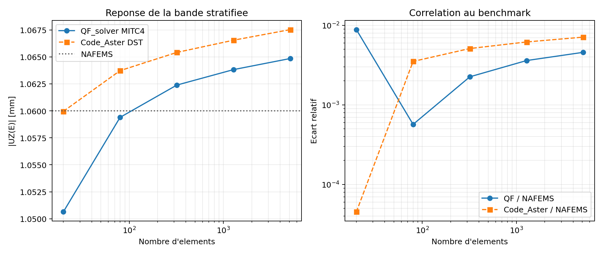
Cook, Scordelis–Lo, pinched-cylinder, modal-plate, Newmark, harmonic, and laminate cases have separate records.
Each reference supports its own model, observable and analysis route. Read the original contract and limitations before transferring a conclusion.
See this method in a calculation.
Each case keeps its mesh, measured quantities, source record and limitations attached to the result.