
A complete white-box walk-through of the four-node tetrahedron: continuum balance, barycentric interpolation, orientation and gradients, strain convention, constitutive law, stiffness, mass, loads, code, proof checks, and usage limits.
01 Model and scope
A TET4 is a linear tetrahedron with four corner nodes and three translations at each node: 12 element DOFs. Barycentric interpolation reproduces any affine displacement field exactly. Its defining trade-off is that the strain and stress are constant inside each element, then may jump at element faces.
Route assumptions and calculation checks
- Derive the weak form from local equilibrium and prescribed displacement/traction boundaries.
- Map the reference tetrahedron; check signed volume and compute constant physical shape gradients.
- Assemble the 6×12 engineering-strain matrix B and the 12×12 element stiffness Kₑ = V Bᵀ D B.
- Integrate consistent mass and equivalent loads; audit force and moment resultants.
- Verify rigid modes, affine patch response, equilibrium/energy, then named mesh-refinement trends.
Useful foundations and prerequisites
02 Essential equations and symbols
Definitions and conventions
- Barycentric shape function of node i.
- Maps the element displacement vector to engineering strain.
- Constitutive matrix in the declared Voigt order.
- Physical volume after the signed-orientation check.
03 Step by step derivation
Follow the assumptions, equations and discrete operations in order. The full explanation stays visible.
The sheet follows the complete chain: continuum equilibrium → weak form → barycentric interpolation → physical gradients → engineering-strain matrix B → constitutive matrix D → element stiffness, mass, and loads. The formula Kₑ = V BᵀDB is exact for a straight, non-degenerate tetrahedron with constant B and homogeneous linear-elastic D; it is not a claim of exactness for an entire discretized structure.
1 · Start with the continuum problem
For small-strain quasi-static elasticity, the unknown is displacement. The strong form expresses local force balance; prescribed displacement is imposed on Γu and prescribed traction on Γt. The Cauchy stress follows the material law. Multiplying equilibrium by a virtual displacement and integrating by parts transfers one spatial derivative from stress to the test function. This weak form is the starting point for finite elements.
2 · Interpolate displacement with four barycentric functions
On the reference tetrahedron, r, s, t are non-negative and r+s+t≤1. Each barycentric shape function is one at its own vertex and zero at the other three. Their sum is one, so a constant nodal displacement remains constant everywhere; the coordinate reproduction identity makes every affine field exact. The element displacement vector is ordered node by node as (ux, uy, uz). There are no rotational DOFs.
A rigid rotation is represented by nodal translations dₐ = ω × xₐ. The formulation does not assign independent nodal rotations.
3 · Map the reference cell and check its orientation
For a straight-sided TET4 the map is affine, so the Jacobian is constant. The determinant gives six times the signed physical volume. QF Solver rejects a degenerate or negatively oriented cell; silently taking |det A| would hide a connectivity error. Gradients in physical coordinates are constant and can be computed once per element.
Worked geometry check: for vertices (0,0,0), (1,0,0), (0,1,0), (0,0,1), det(A)=1 and Vₛ=1/6. The shape functions are 1−x−y−z, x, y, z. A different node ordering can change the sign; the code tests signed_volume before constructing stiffness.
4 · Build B using engineering shear strain
Collect the six independent strain components in the order [εxx, εyy, εzz, γxy, γyz, γzx]. The last three entries are engineering shears (γxy=2εxy), not tensor shear strains. This convention must match D; otherwise shear stiffness is wrong by a factor of two. For node a, let (bₐ,cₐ,dₐ) be the x, y, z derivatives of Nₐ. The four 6×3 blocks form a 6×12 matrix.
For the worked unit tetrahedron, ∇N₁=(−1,−1,−1), ∇N₂=(1,0,0), ∇N₃=(0,1,0), ∇N₄=(0,0,1). The code delegates B assembly to the shared strain_displacement_from_gradients routine.
5 · Apply the constitutive law and derive stiffness
For isotropic linear elasticity, D is symmetric and maps engineering strain to stress. The two Lamé constants are derived from Young’s modulus E and Poisson ratio ν. In the discrete virtual-work equation, B and D are constant within a straight TET4 with homogeneous material, so the volume integral reduces to a closed-form product. This is why one integration point is exact here; it is not an arbitrary reduced-integration approximation.
The implementation returns (Kₑ+Kₑᵀ)/2 to remove floating-point asymmetry. For a stable material and non-degenerate tetrahedron, a free element has six rigid-body zero-energy modes; supports remove the corresponding global mechanisms.
6 · Consistent mass and equivalent nodal loads
The consistent mass comes from the same interpolation: Mₑ=∫ρNᵀN dΩ. Integrating products of linear barycentric functions gives twice the diagonal block weight of an off-diagonal block. A uniform body-force density distributes equally to the four vertices. A uniform traction over one triangular face distributes equally to its three nodes. For pressure, the outward-normal convention makes positive pressure compressive.
Summing the diagonal spatial contributions of the consistent mass recovers total mass ρV in each translation direction. Modal analysis also requires strictly positive density in the TET4 implementation.
7 · What the verification demonstrates—and what it does not
Verification is a chain of separate checks, not a single successful run. Unit tests check volume, gradients, symmetry, mass and invariants. A free-element check detects the six rigid modes. An affine patch checks interpolation plus assembly and stress recovery. Analytical traction/compression and load audits check signs and global balance. Mesh refinement checks convergence trends for named examples. These tests support only their recorded observables and parameter domain.
The source excerpt is pinned to public tag v0.2.11, but the maturity label on this card comes from the named v0.2.8 registry records; a later package release does not automatically requalify a route. The cited qualification domain is narrower than every mathematically admissible elastic law: isotropic 3D, E>0, and 0≤ν≤0.45 for the recorded TET4 linear-static route. The element’s small-strain class and constitutive tangent pathway do not qualify every nonlinear material, geometric-nonlinear route, solver, or contact combination.
8 · Limits that matter in practice
Because strain is constant per element, bending-dominated response and steep stress gradients need mesh refinement; raw stress can jump across faces. Point stresses at singularities do not converge in the same way as global displacements or energy. As ν approaches 0.5, the displacement TET4 can volumetrically lock and become too stiff. Sliver tetrahedra worsen matrix conditioning. Smoothed nodal stress is a visualization recovery, not a new equilibrated finite-element solution.
04 Algorithm and implementation
Source excerpt · v0.2.11
These excerpts from v0.2.11 show both the linear-elastic stiffness and the constitutive trial-state/internal-force tangent path. The second path does not by itself qualify every nonlinear material or solver combination.
Functions shown: stiffness internal_force_tangent_state
def stiffness(self, coords):
    coords = validate_coords_shape(coords, (4, 3), "TET4")
    volume = self.signed_volume(coords)
    if volume <= 1.0e-14:
        raise ValueError(f"Invalid TET4 volume {volume:.6e}.")
    b = self.strain_displacement_matrix(coords)
    ke = volume * (b.T @ self.material.elasticity_matrix @ b)
    return symmetrize(ke)

def internal_force_tangent_state(
    self, coords: np.ndarray, local_displacement: np.ndarray,
    states: list[dict[str, object]] | None = None,
):
    volume = self.signed_volume(coords)
    if volume <= 1.0e-14:
        raise ValueError(f"Invalid TET4 volume {volume:.6e}.")
    b = self.strain_displacement_matrix(coords)
    strain = b @ np.asarray(local_displacement, dtype=float)
    updated_states = []
    previous = states[0] if states else None
    response = evaluate_constitutive(self.material, strain, previous)
    stress, tangent = response.stress, response.tangent
    if response.diagnostics.get("stateful", False):
        updated_states.append(response.trial_state)
    internal = volume * (b.T @ stress)
    stiffness = volume * (b.T @ tangent @ b)
return internal, symmetrize(stiffness), updated_states05 Verification and limitations
QUALIFIED_BOUNDED · recorded 0.2.8 routes
One-element tensile/compressive test, affine patch test, and refinement examples.
Each reference supports its own model, observable and analysis route. Read the original contract and limitations before transferring a conclusion.
See this method in a calculation.
Each case keeps its mesh, measured quantities, source record and limitations attached to the result.
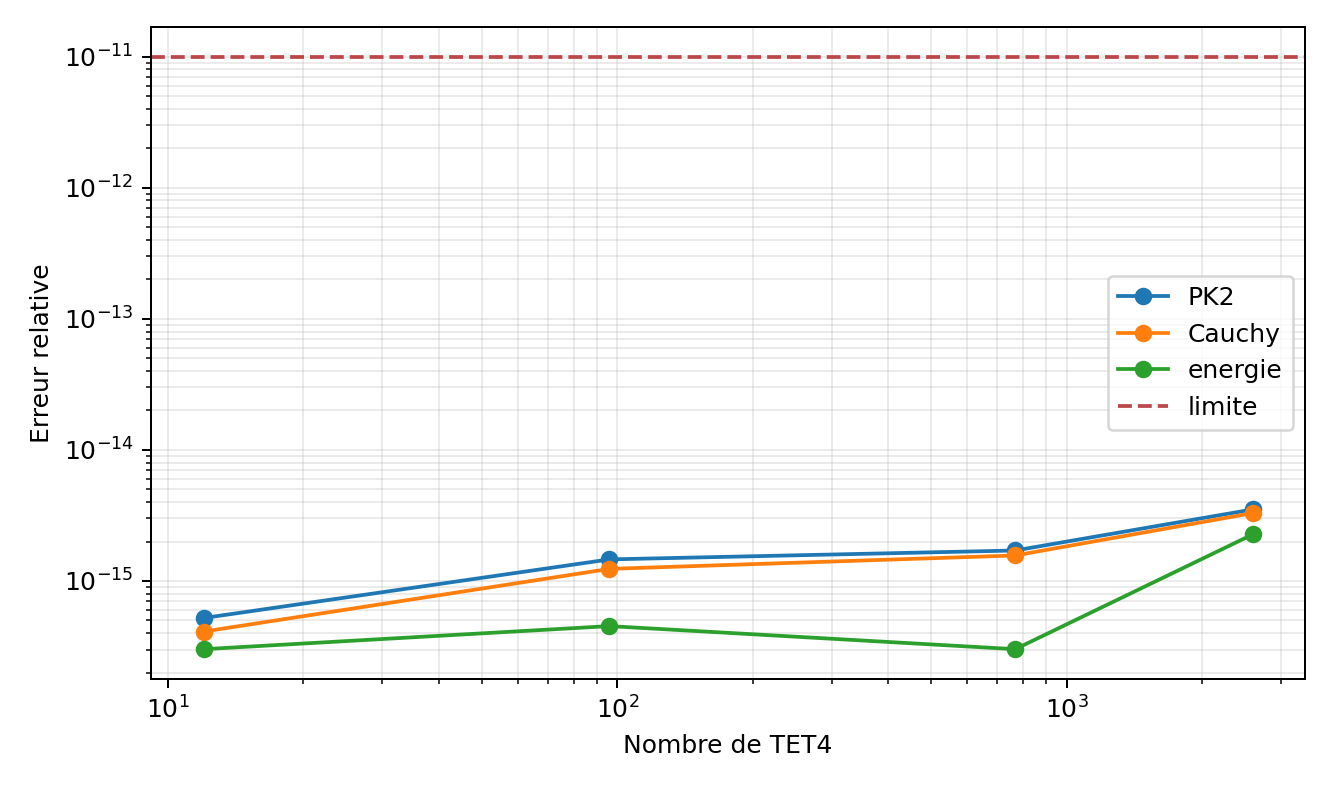 VNV-TET4-TL-STRESS-001TET4 affine finite-strain patchObserved patch error: ≈ 10⁻¹⁵Read model, result and limits →
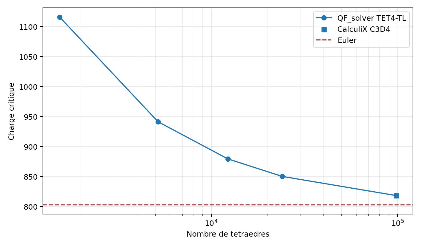 VNV-TET4-TL-BUCKLING-002TET4 linearized buckling refinementQF Solver critical load: 818.415402Read model, result and limits →
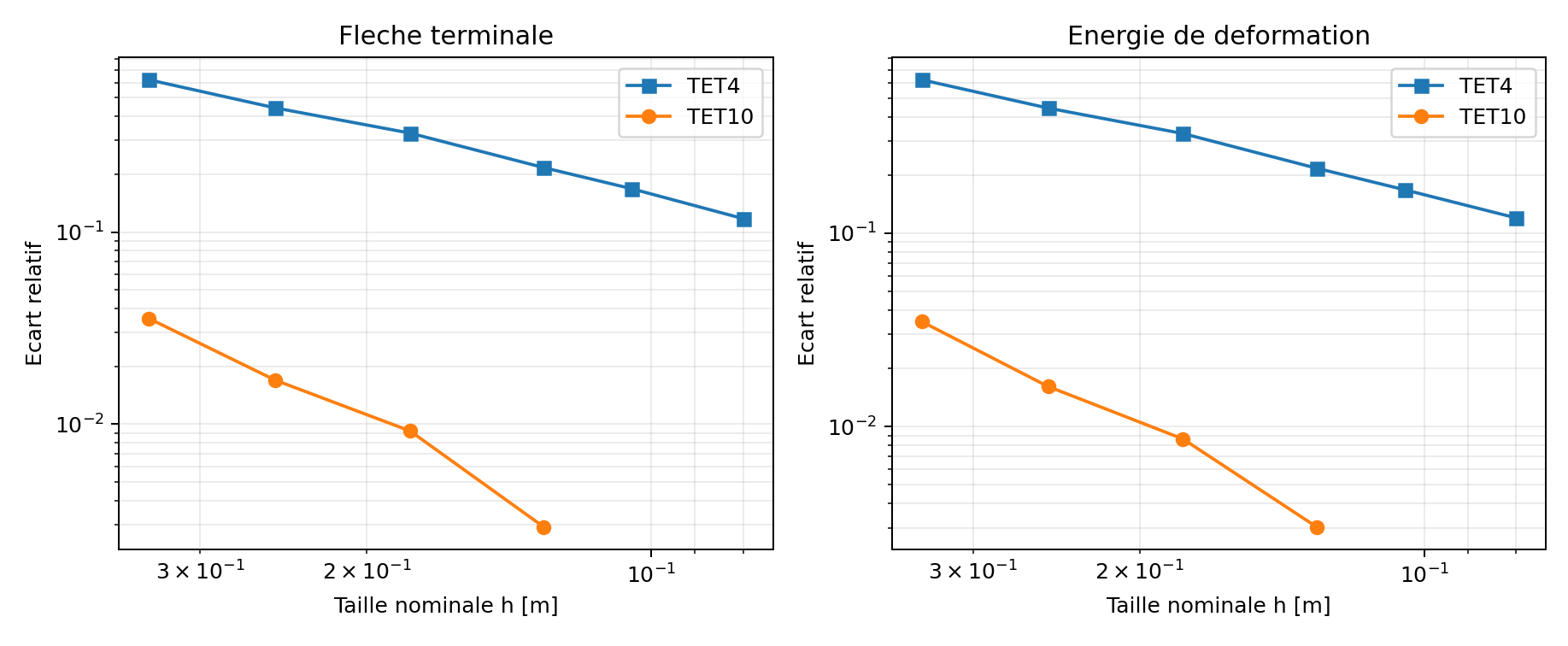 VNV-ORTHOTROPIC-SOLID-CONVERGENCE-003Orthotropic solid mesh convergenceTET10 deflection error: 0.292%Read model, result and limits →
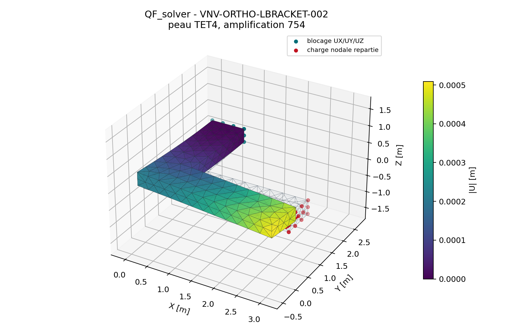 VNV-ORTHOTROPIC-SOLID-EXTERNAL-002Orthotropic bracket and perforated specimen correlationPerforated field difference: 0.000132% / 3.60 × 10⁻¹¹%Read model, result and limits →