
Ten-node isoparametric solid with four corner nodes, six midside nodes, and thirty translational DOFs. Straight-sided cells use four-point Hammer stiffness integration; curved cells switch to a 64-point Duffy rule, while consistent mass uses 125 points.
01 Model and scope
Quadratic corner and edge functions interpolate both the curved geometry and displacement field. The chain rule maps reference derivatives to physical gradients through J⁻ᵀ; stiffness then integrates the resulting spatially varying B over the element.
Route assumptions and calculation checks
- The geometry and displacement use the same quadratic basis; the six edge-node positions control whether the geometry is straight or curved.
- The implementation selects four-point Hammer stiffness integration for straight-sided cells and 64-point Duffy integration for curved cells; consistent mass uses a separate 125-point rule.
- Jacobian sign is checked at a closed sample lattice and at integration points; this is a strong diagnostic, not an analytic proof of positivity everywhere.
Useful foundations and prerequisites
02 Essential equations and symbols
Definitions and conventions
- Lᵢ
- Barycentric coordinate at corner i.
- Nᵢ, Nᵢⱼ
- Quadratic corner and edge shape functions.
- Jacobian of the isoparametric geometry map.
- w_g, det(J_g)
- Quadrature weight and local volume scale at point g.
03 Step by step derivation
Follow the assumptions, equations and discrete operations in order. The full explanation stays visible.
At each integration point, J = ∂x/∂ξ maps parent coordinates to physical space. The chain rule gives ∇ₓN = J⁻ᵀ∇ξN, then B is assembled from these physical gradients. The local energy is integrated as Kₑ = Σg w_g det(J_g) B_gᵀ D B_g. Curvature makes J and B vary within the cell, so a valid Jacobian and adequate quadrature are essential.
1 · Ten nodes and the quadratic tetrahedral basis
TET10 adds one node at the midpoint of each of the six edges to the four TET4 corners. The documented local edge order is (1,2), (2,3), (3,1), (1,4), (2,4), (3,4); this ordering is part of the mesh-connectivity contract. Each node carries three translations, so the element vector has 30 entries.
Permuting midside nodes changes both geometry and displacement interpolation. It is not just a display-order issue.
2 · Isoparametric geometry and displacement
The same quadratic shape functions map the reference tetrahedron into the physical cell and interpolate displacement. This lets the midside coordinates represent curvature. If all midside points lie exactly on straight edges, the geometry is straight even though the displacement basis remains quadratic.
For an affine geometry map the quadratic basis reproduces quadratic displacement fields. Curved geometry introduces a varying Jacobian and changes the physical gradients at every integration point.
3 · Physical gradients, strain, and the stiffness integral
At each quadrature point the implementation computes the Jacobian, rejects a non-positive determinant, maps reference derivatives into physical derivatives, then builds the same engineering-shear B convention as TET4. Unlike TET4, B and det(J) generally vary through the cell, so stiffness is a weighted sum rather than a single volume product.
Straight-sided cells use the four-point Hammer degree-two rule. Curved cells switch to a positive 64-point Duffy rule of order four; the 125-point Duffy rule belongs to consistent mass. A closed 35-point barycentric Jacobian sample detects bad geometry, but sampling is not an analytic proof that det(J)>0 everywhere.
4 · Consistent mass and quadratic face loads
The consistent mass is the integral of the interpolated velocity field, including off-diagonal coupling between the ten nodes. The implementation uses 5×5×5=125 Duffy/Gauss points for this volume integral. A quadratic triangular face has three corners and three midside nodes; a uniform traction can therefore assign zero force to corner nodes and nonzero equivalent force to midside nodes without losing resultant or moment.
Positive density is required for the modal mass. The face rule and the geometry map are part of the load calculation, not just the solid stiffness kernel.
5 · What the verification results say
Element checks cover partition of unity, derivatives, six rigid modes, stiffness symmetry and energy, mass positivity, aligned and oblique affine patches, quadratic-field recovery, and Gmsh reorientation. Structural cases then probe bending, curved-cylinder Lamé response, modal frequencies, loads, and same-mesh external correlation. In the cited four-level bending campaign, final compliance error was 45.75% for TET4 and 1.179% for TET10; that is one benchmark sequence, not a universal accuracy ratio.
Evidence is observable-specific. For example, the curved-cell quadrature error compares against an order-eight Duffy reference; it does not establish every mesh, constitutive law, or nonlinear solve.
6 · Limits and route boundaries
Quadratic interpolation improves representation but does not remove the need for mesh quality, integration checks, or refinement. Curved midside placement must be geometrically intentional. Stress recovery between integration points is post-processing. The documented stateful nonlinear route currently stores states at the Hammer points; the curved-geometry enriched stiffness rule is outside that stateful quadrature path. Read the exact registry row before transferring evidence to nonlinear, modal, or contact combinations.
04 Algorithm and implementation
Source excerpt · v0.2.11
At each quadrature point, reference derivatives form the Jacobian. Its inverse maps gradients into physical coordinates; non-positive Jacobians are rejected.
dnr = cls.shape_derivatives_reference(barycentric)
jacobian = dnr.T @ coords
det_j = float(np.linalg.det(jacobian))
if det_j <= 1.0e-14:
    raise ValueError(f"Invalid TET10 jacobian {det_j:.6e}.")
gradients = dnr @ np.linalg.inv(jacobian).T
return strain_displacement_from_gradients(gradients), det_j05 Verification and limitations
QUALIFIED_BOUNDED · nonlinear extensions remain narrower
Quadratic patch, curved-cylinder Lamé benchmark, and recorded linear/J2 cases.
Each reference supports its own model, observable and analysis route. Read the original contract and limitations before transferring a conclusion.
See this method in a calculation.
Each case keeps its mesh, measured quantities, source record and limitations attached to the result.
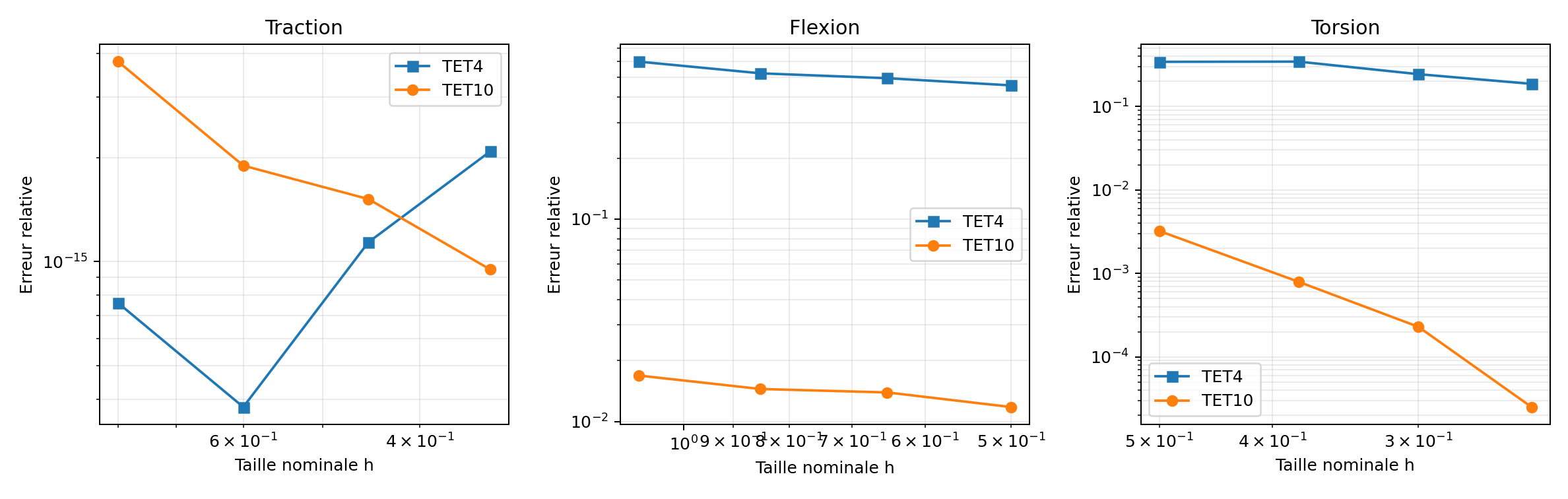 VNV-TET10-STRUCTURAL-CONVERGENCE-012TET10 structural mesh convergenceTET10 bending error: 1.179%Read model, result and limits →
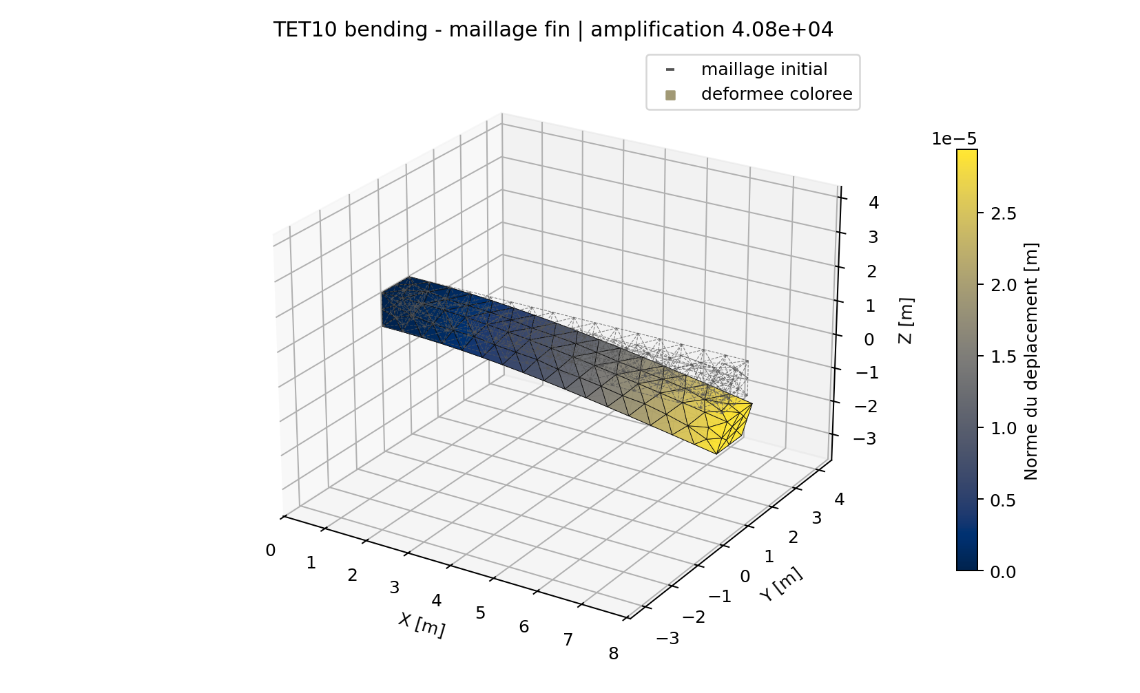 VNV-TET10-STRUCTURAL-CONVERGENCE-012-BTET10 cantilever bending shapeDisplay amplification: 40,800×Read model, result and limits →
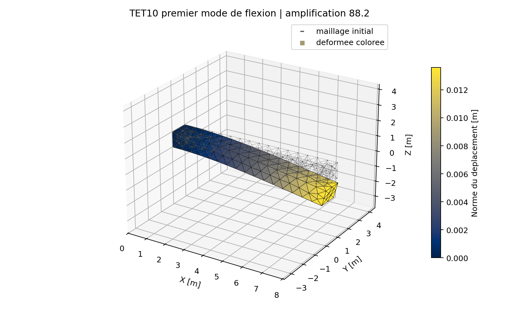 VNV-TET10-MASS-MODAL-LOADS-013-MTET10 first bending modeFirst bending frequency pair: 12.7961 / 12.7965 HzRead model, result and limits →
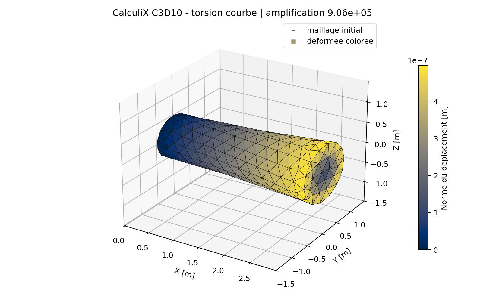 VNV-TET10-CALCULIX-C3D10-014TET10 torsion field correlation with CalculiXRelative full displacement field difference: 6.84 × 10⁻⁵Read model, result and limits →