Arc-length continuation

Algorithm / executionEXPERIMENTAL_BOUNDED · no general postbuckling claim

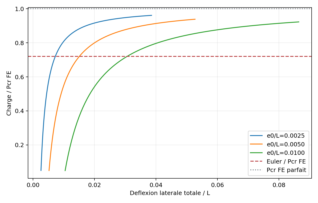
The load factor is an unknown alongside displacement so a declared equilibrium branch can be followed through bounded increments.

01 Model and scope

The implemented custom spherical continuation solves free displacement and load factor together. A spherical condition closes equilibrium, while predictor orientation, acceptance, rollback and radius control govern how the next state is attempted.

Route assumptions and calculation checks

The route has specialized correction logic and is not identical to load-control Full Newton.
Evidence does not establish general limit-point tracking, bifurcation handling, imperfection sensitivity, or postbuckling.
Use only the frozen element, loading, imperfection, and step controls for the demonstrated case.

Useful foundations and prerequisites

Full Newton with line search Accepted and trial material state

02 Essential equations and symbols

\mathbf R(\mathbf u,\lambda)=\lambda\mathbf f_{ref}-\mathbf f_{int}(\mathbf u)

Definitions and conventions

$\mathbf R(\mathbf u,\lambda)$: External minus internal force residual.
$\Delta\mathbf u,\Delta\lambda$: Full trial-step increments from the last accepted base.
$\delta\mathbf u,\delta\lambda$: Corrector increments within the current arc step.
$\alpha,s$: Declared load-factor scale and attempted spherical radius.
$d$: Signed predictor orientation.
$R_{ref},g_{ref},\tau$: Source-defined residual scale, constraint scale and nonlinear acceptance tolerance.

Equilibrium branch and arc constraintConceptual drawing in scaled displacement and load coordinates. The constraint closes the augmented problem. This is not a computed branch or evidence of postbuckling validity.

6 detailed steps

03 Step by step derivation

Follow the assumptions, equations and discrete operations in order. The full explanation stays visible.

1 · Define the accepted base and unknowns

The implemented residual is external minus internal force. Measure the trial step from the last accepted displacement and load factor. Displacement and load factor are solved together. The arc route is exposed through nonlinear_static, not as an automatic property of every geometric nonlinear analysis.

\mathbf R=\lambda\mathbf f_{ref}-\mathbf f_{int}(\mathbf u)

2 · Close the problem with the implemented spherical metric

The custom spherical constraint uses the Euclidean free-displacement increment and a declared load-factor scale α. The radius s belongs to this scaled displacement/load space. The predictor solves the current tangent against the reference load direction, then normalizes the augmented increment.

g=\Delta\mathbf u^T\Delta\mathbf u+\alpha^2\Delta\lambda^2-s^2

The contract names this route SPHERICAL_ARC_LENGTH_CUSTOM. It does not establish equivalence to a named Riks or Crisfield implementation.

3 · Solve the actual augmented corrector

Linearize equilibrium and the spherical condition with respect to correction increments δu and δλ. With the external-minus-internal residual convention, the top right-hand side is R and the constraint right-hand side is −g. The kernel preserves a sparse CSC block matrix and calls SciPy spsolve.

\begin{bmatrix}\mathbf K_{ff}&-\mathbf f_{ref,f}\\2\Delta\mathbf u^T&2\alpha^2\Delta\lambda\end{bmatrix}\begin{bmatrix}\delta\mathbf u\\\delta\lambda\end{bmatrix}=\begin{bmatrix}\mathbf R_f\\-g\end{bmatrix}

The augmented system is generally nonsymmetric. CG/MINRES or a distributed backend cannot inherit this correction route without a separate contract.

4 · Check equilibrium and the arc constraint together

The current acceptance value is the maximum of normalized free residual and normalized spherical-constraint error. The recorded source uses max(norm(reference load), 1.0) for the force reference and max(s², 1.0e−30) for the constraint reference in the declared unit system. These are implementation normalizations. The current arc loop has no separate correction-magnitude acceptance gate.

\rho=\max\left(\frac{\|\mathbf R_f\|}{R_{ref}},\frac{|g|}{g_{ref}}\right)

Do not infer the Newton sheet's general increment checks as an additional acceptance gate in this specialized arc route.

5 · Preserve branch orientation and rollback

A signed predictor follows the declared load direction and then uses previous displacement orientation, with a scaled augmented tie-breaker. Rejection restores the accepted state before radius reduction or retry. Target clipping and adaptive-radius policies are distinct from the spherical constraint itself.

\mathbf S_{n+1}=\begin{cases}\mathbf S^*,&\mathcal C=1\\\mathbf S_n,&\mathcal C=0\end{cases}

A direction policy is not evidence of branch switching, general bifurcation handling or imperfection robustness.

6 · Bound the reported result

Record the reference load, accepted base, radius and scale, displacement and load-factor increments, equilibrium and constraint errors, iteration count and rejected retries. The linked contract is a technical candidate tied to its original source revision. It does not establish structural postbuckling qualification or external validation.

Read the original contract and readiness review alongside the v0.2.11 correction source. The contract preserves its historical review status.

04 Algorithm and implementation

Source excerpt · v0.2.11

Core assembly excerpt from solve_arc_length_correction at v0.2.11. The complete function includes shape checks, singular-system handling and non-finite result rejection. Its right-hand side uses external-minus-internal residual and minus the spherical constraint.

matrix = bmat(
    [
        [csr_matrix(tangent), csc_matrix((-reference_load).reshape(size, 1))],
        [csr_matrix((2.0 * delta_u_step).reshape(1, size)), csc_matrix([[2.0 * load_scale**2 * delta_lambda]])],
    ],
    format="csc",
)
rhs = np.concatenate((np.asarray(residual, dtype=float), np.asarray([-constraint], dtype=float)))
solution = spsolve(matrix, rhs)

Read the complete versioned implementation →

Sparse augmented correction implementation

05 Verification and limitations

EXPERIMENTAL_BOUNDED · no general postbuckling claim

Each reference supports its own model, observable and analysis route. Read the original contract and limitations before transferring a conclusion.

Arc-length formulation contract Readiness review

Recorded repository calculations

See this method in a calculation.

Each case keeps its mesh, measured quantities, source record and limitations attached to the result.

Three TET4 postbuckling load-deflection paths for different initial imperfections.

VNV-TET4-TL-POSTBUCKLING-003TET4 imperfect postbuckling pathsInitial imperfection amplitudes: 0.0025 / 0.005 / 0.01Read model, result and limits →

Browse every calculation case →

06 Sources and related sheets

Sparse augmented correction implementation Arc-length formulation contract Readiness review

Continue the reasoning

Full Newton with line search Accepted and trial material state

Back to sheet contents ↑